Gene Ontology, or GO, is a massive bioinformatics project designed to create a common language for describing how genes and their products behave across all species. Think of it as a meticulously organized dictionary that gives scientists a standardized, computer-readable way to talk about what genes do, where they do it, and what larger processes they're involved in. This structure is what allows researchers to consistently analyze and compare huge amounts of genomic data.

What Is Gene Ontology and Why It Matters

Imagine you're building a complex engine with parts from a dozen different suppliers. One calls a part a "piston," another calls it a "plunger," and a third insists it's an "actuator rod." You'd be stuck. This is precisely the problem Gene Ontology solves for the world of genomics—it acts as the universal translator for gene functions.

The whole effort is spearheaded by the Gene Ontology Consortium, a collaborative group that maintains and develops this shared framework.

Before GO came along, functional descriptions were all over the place. It was a chaotic landscape that made it nearly impossible to programmatically compare results from different studies or databases. Launched in 1998 from a collaboration focused on just three model organisms, the GO project introduced the structure that genomics desperately needed.

Today, it’s an indispensable resource, containing over 47,000 terms and more than 1 billion annotations that connect genes to these terms across thousands of species. The project's foundational impact is clear, as shown by the high citation count of its original paper.

The Three Pillars of Gene Function

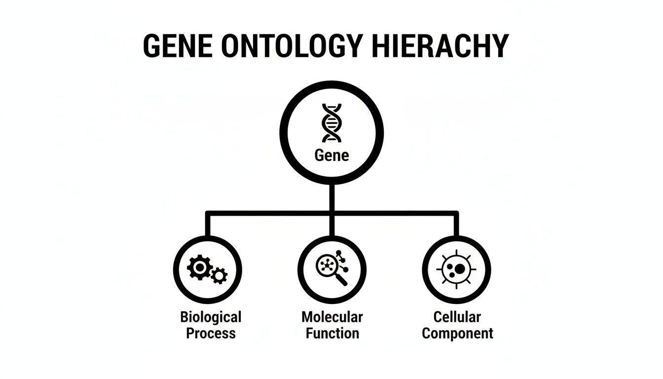
To build this common language, GO organizes everything into three distinct categories, or "ontologies." This structure is key because it ensures every piece of information is precise and has the right context. Getting a handle on these three domains is the first step to putting GO to work.

Let's break down the three core domains of Gene Ontology to see how they provide a comprehensive view of a gene product's role.

The Three Core Domains of Gene Ontology

Domain	What It Describes	Example Term
Molecular Function (MF)	The specific biochemical job of a gene product at the molecular level. Think of it as the gene's "job title."	"protein kinase activity" or "DNA binding"
Biological Process (BP)	The larger biological goal or pathway the gene product contributes to. This is the "project" the gene works on.	"cell division" or "signal transduction"
Cellular Component (CC)	The specific location within a cell where the gene product is active. This is the gene's "workplace."	"nucleus" or "plasma membrane"

This clear separation allows for a much richer, multi-faceted understanding. A single gene product can, and often does, have multiple annotations across all three domains, painting a complete picture of its function in biology.

By separating these three aspects, Gene Ontology allows for a multi-faceted view of a gene's role. A single gene product can have multiple annotations across all three domains, painting a complete picture of its contribution to biology.

For data engineers and developers, this standardized framework is a game-changer. It’s the common vocabulary you need to make sense of massive genomic datasets, compare experimental results, and reliably integrate functional data into complex OMOP pipelines. If you're building out your foundational knowledge, our guide on medical terminology might also be a useful resource. Ultimately, this structured approach is what enables the advanced analytics and machine learning applications that depend on consistent, high-quality biological data.

Decoding the Structure of Gene Ontology

To really get a handle on Gene Ontology, you have to look past what it is and dig into how it's built. GO isn't just a massive, flat list of biological terms; it’s a sophisticated structure called a Directed Acyclic Graph (DAG). This graph format is precisely what gives GO its analytical horsepower, enabling complex queries and a much more nuanced view of biological data.

Think of it like a family tree, but with a clever twist. In a normal family tree, a child has exactly two parents. In GO's DAG, a specific term (the "child") can have multiple parent terms. This creates a rich, interconnected web where a highly specific term can inherit traits and relationships from several broader concepts at once.

This structure ensures that every term eventually traces back to one of the three core domains: Molecular Function, Biological Process, or Cellular Component. This organization is key, as it provides a clear and distinct context for every single annotation.

The Relationships That Build the Graph

The connections in this graph aren't random; they're defined by very specific relationship types. These relationships are the logical glue holding the whole ontology together, allowing a computer to understand how one biological concept relates to another. Getting these relationships straight is fundamental to navigating the GO structure.

The two most common and important relationships are:

is_a: This is a classic parent-child relationship. For instance, "mitochondrion" is_a "intracellular membrane-bounded organelle." This means anything that holds true for the parent term is automatically true for the child.
part_of: This one is pretty intuitive. It indicates that a child term is a physical component of a larger parent term. A great example is the "mitochondrial inner membrane," which is part_of the "mitochondrion."

These relationships create clear paths from the most granular terms at the bottom of the hierarchy all the way up to the very general ones at the top. The multi-parent nature of the DAG means a single term can be connected to the top through several different paths, creating a dense web rather than a simple tree. This is the defining feature of the DAG and what makes it so powerful.

A Practical Example of the DAG

Let’s trace a real-world example to see this in action. We'll use the specific molecular function GO:0005524, which stands for "ATP binding."

"ATP binding" is_a "adenyl ribonucleotide binding."
"Adenyl ribonucleotide binding" is_a "adenyl nucleotide binding."
"Adenyl nucleotide binding" is_a "purine nucleotide binding."
…and so on, until you eventually reach the top-level parent term, "Molecular Function."

By following these is_a links, a program can logically infer that a gene annotated with "ATP binding" is also involved in "purine nucleotide binding." You simply can't achieve this kind of reasoning with a flat file.

For developers, the DAG is the blueprint for programmatic traversal. Understanding this structure is essential for mapping genomic data into structured models like OMOP, as it enables the nuanced, hierarchical queries that drive powerful analytics.

This ability to move up and down the hierarchy is what allows researchers to perform enrichment analysis—a technique we'll cover later—where they can identify broader functional patterns from a list of specific genes.

Developer Tips for Working with the GO Structure

Use the Right Tools: Don't even think about parsing the raw GO files manually. There are well-established libraries in Python and R specifically designed to traverse the DAG structure efficiently.
Understand Relationship Types: While is_a and part_of are the most common, other relationships like regulates exist. Knowing which relationships to follow is critical for your specific analysis.
Lean on OMOPHub: If you're integrating GO into an OMOP environment, a managed vocabulary platform can save you a world of headaches. The OMOPHub Python and R SDKs provide functions to programmatically explore these relationships without the pain of managing the underlying database. You can find more details in the official documentation. This approach saves a ton of development time and guarantees your vocabulary data is always current.

Understanding GO Annotations and Evidence Codes

The Gene Ontology's hierarchical structure gives us a detailed map of biology, but the real magic happens when we connect specific genes to terms on that map. That connection is an annotation—a formal statement linking a gene product to a GO term, effectively claiming it plays a role in a certain process, has a particular function, or resides in a specific cellular location. But in science, any claim is only as good as the evidence backing it up.

This is where evidence codes come into play, and frankly, they are critical. An evidence code is a simple, three-letter tag attached to every GO annotation that tells you the story behind the claim. It answers the fundamental question: "How do we know this gene does this?" For anyone building clinical-grade data pipelines or running high-stakes research, paying attention to these codes isn't optional. They are your primary tool for judging the quality and reliability of the data you're working with.

Over the last two decades, Gene Ontology has become a cornerstone of genomic standards. It’s seen relentless growth in its terms, annotations, and real-world impact. For instance, in 2014 alone, terms related to kidney development jumped by 522 new entries with 940 new protein annotations. Today, the resource supports over 1 billion gene-term associations across countless species. You can dig into the full history of these gene ontology expansions and their impact to see just how far it's come.

Differentiating Strong from Weaker Evidence

Not all evidence is created equal, and GO evidence codes are what allow us to see the difference. They let you distinguish between annotations backed by direct lab experiments and those that are essentially educated guesses from a computer. For any serious analysis, knowing the difference is vital.

The most trustworthy annotations come directly from experimental results. These are the gold standard because they’re derived from someone in a lab coat specifically investigating that gene product.

IDA (Inferred from Direct Assay): This code means a function was shown through a direct biochemical experiment. Think of a scientist purifying a protein and running an assay that proves it can bind to ATP. That's IDA.
IMP (Inferred from Mutant Phenotype): Here, the proof comes from seeing what happens when you break the gene. If deleting a gene halts cell division, that’s powerful evidence the gene is involved in that process.

On the other end of the spectrum are annotations generated by automated, computational methods. They are incredibly useful for annotating entire genomes at scale, but it's important to remember they are predictions, not direct observations.

IEA (Inferred from Electronic Annotation): This is by far the most common code you'll see. It means the annotation was made automatically by a computer program, usually by noticing a gene's sequence looks a lot like another well-studied gene. It's a powerful tool for discovery, but it carries a much lower level of confidence.

Why Evidence Codes Matter in Practice

Let’s make this concrete. Imagine you're building a machine learning model to predict how a patient might respond to a drug targeting a specific biological pathway. If you train that model using gene sets full of IEA annotations, you're building your model on a foundation of predictions. If just one of those initial computational predictions was off, that error could cascade through your entire analysis and lead to some seriously flawed conclusions.

By filtering your dataset to include only annotations with strong experimental evidence codes like IDA or IMP, you can significantly increase the confidence in your results. This is a critical step for building high-confidence datasets, especially in regulated or clinical environments.

A common workflow I see is to run an initial, broad exploratory analysis using all available evidence codes. Then, to validate the most interesting findings, you'd repeat a much more stringent analysis using only the experimentally verified annotations. This two-step approach gives you the best of both worlds: broad discovery without sacrificing scientific rigor.

Understanding the different evidence codes is key to this process. While there are over 20 codes, they fall into a few main categories that tell you where the information came from.

Common Gene Ontology Evidence Codes

This table breaks down some of the most frequently encountered GO evidence codes, grouping them by the type of evidence they represent. It's a handy reference for quickly assessing the foundation of a given annotation.

Code	Name	Evidence Type	Description
IDA	Inferred from Direct Assay	Experimental	Evidence from a direct biochemical or physical experiment on the gene product (e.g., an enzyme assay).
IMP	Inferred from Mutant Phenotype	Experimental	Evidence from observing the outcome of mutating the gene (e.g., a knockout mouse shows a specific defect).
IGI	Inferred from Genetic Interaction	Experimental	Evidence from genetic experiments where one gene's function is modified by another (e.g., synthetic lethality).
IPI	Inferred from Physical Interaction	Experimental	Evidence from protein-protein interaction studies (e.g., yeast two-hybrid or co-immunoprecipitation).
ISS	Inferred from Sequence or Structural Similarity	Computational	A curator infers function based on sequence/structural similarity, but it is not an automated process.
IEA	Inferred from Electronic Annotation	Computational	Annotation is automatically assigned by a computational method without human review. The most common code.
TAS	Traceable Author Statement	Author Statement	Evidence comes from a statement in a published paper that the curator has reviewed and verified.
NAS	Non-traceable Author Statement	Author Statement	Evidence is based on a statement in a publication, but it's not traceable to a specific experiment.

Knowing whether an annotation stems from a direct lab result (like IDA or IMP) versus an automated prediction (IEA) lets you set the right level of confidence for your own work.

Tips for Integrating GO Evidence Codes

Filter by Evidence Type: When you're running an enrichment analysis, most tools give you the option to filter annotations by their evidence codes. As a first step, try excluding IEA annotations to see how much it changes your results. You might be surprised.
Check Annotation Sources: Always be mindful of where your annotations are coming from. Different curation groups and databases can have different standards or focus areas.
Programmatic Access with OMOPHub: For developers pulling GO into an OMOP CDM, managing these details can get complicated fast. The OMOPHub SDKs make this much easier by giving you programmatic ways to access vocabulary details, including annotation evidence. You can explore how to query these relationships in the OMOPHub documentation. To get started, check out the SDKs for Python and R on GitHub.

Performing Gene Ontology Enrichment Analysis

So, you’ve run your experiment—maybe an RNA-seq study—and you have a list of interesting genes. Perhaps they're all upregulated in patients with a specific disease. That’s a great start, but it’s just a list. The real question is: what do these genes actually do together?

This is where Gene Ontology (GO) enrichment analysis comes in. It's the standard, go-to method for turning a simple gene list into a coherent biological story. It’s a statistical technique that helps you see the forest for the trees.

The core idea is simpler than it sounds. Imagine you find out that a surprising number of students who aced a tough exam all belong to the same study group. You’d instantly suspect that group was "enriched" with top performers and that their collaboration was key. GO enrichment does the same thing, just with genes. It scans your list and asks: are any specific biological functions, components, or processes (the GO terms) showing up way more often than you’d expect by random chance?

This is how you move from a list of individual genes to identifying the major biological themes at play, like "immune response" or "apoptotic process." It's about finding the bigger picture hidden in your data.

The Core Workflow of Enrichment Analysis

While the math behind it can get a little dense, the actual workflow is pretty straightforward. Following established data analysis best practices is crucial here to make sure your results are both reliable and meaningful.

Here’s how it usually breaks down:

Start with a Gene List: This is your input. It’s the set of gene identifiers from your experiment that you suspect are biologically important.
Define a Background Set: This step is critical. You can't just compare your list to the entire genome. You need a relevant "universe" of genes, which should be all the genes that were actually measured in your experiment. This provides the proper context for your statistical tests.
Perform Statistical Testing: For every GO term, the analysis tool counts how many of your genes are annotated with that term. It then compares this count to how many you'd expect to see just by chance, given the background set. This usually involves a statistical test like Fisher's exact test.
Correct for Multiple Testing: Here’s a trap for the unwary. You're testing thousands of GO terms at once, which means you're guaranteed to get some false positives. Applying a statistical correction, like the Benjimini-Hochberg method to control the False Discovery Rate (FDR), is non-negotiable for producing robust results.
Interpret the Results: The final output is a ranked list of GO terms, typically sorted by their corrected p-value (often called a q-value). The terms at the top of the list, with the smallest values, are the biological themes most significantly overrepresented in your gene list.

Choosing the Right Tools and Avoiding Pitfalls

Plenty of great tools can run this analysis for you. Web-based platforms like PANTHER and DAVID are popular, as are programmatic packages like topGO for the R programming language. They do the heavy lifting of mapping genes to terms and running the stats.

But even with the best tools, it's easy to make mistakes that can completely invalidate your findings.

One of the most common errors I see is choosing the wrong background gene set. If you ran your experiment on a microarray that only covers a subset of the genome, you must use only the genes on that array as your background. Using the entire genome as your reference in this case will hopelessly skew your statistics and lead you to the wrong conclusions.

Another layer to consider is the GO hierarchy itself. It’s not just a flat list; it has a structure. Interestingly, researchers have shown that GO terms have an evolutionary history. High-level, ancient functions like "catalytic activity" appeared much earlier than more specialized terms. For a biostatistician, this can be an important analytical lens. If you see an overrepresentation of ancient metabolic GO terms in a disease dataset, it might point to a disruption of very old, fundamental biological pathways.

Practical Tips for Better Enrichment Analysis

To really get the most from your analysis, here are a few things I always keep in mind.

Filter by Evidence Code: Remember those evidence codes we talked about? Not all annotations are created equal. If you want to be extra rigorous, you can run your analysis using only annotations backed by experimental evidence. This can really increase your confidence in the results.
Visualize the Results: A giant spreadsheet of GO terms and p-values is overwhelming. Use tools that can generate a graph or tree visualization. This helps you see the relationships between the enriched terms and makes the story much easier to tell.
Simplify Redundant Terms: You'll often get a cluster of very similar, related terms in your results (e.g., "regulation of transcription," "positive regulation of transcription"). Good analysis tools can help condense these into a single, representative parent term, cleaning up the output and clarifying the core biological message.

Weaving Gene Ontology into Your OMOP Pipeline

This is where the rubber meets the road—connecting the incredible biological detail of Gene Ontology to the structured, real-world data in your OMOP database. It's a massive opportunity, but let’s be honest, it's also a serious technical hurdle. The whole point is to enrich your patient data with functional genomic context, but getting there means wrestling with vocabulary versions, tricky term mappings, and the operational headache of managing another enormous terminology.

This isn’t just an academic exercise. When you get this right, you can build patient cohorts that are vastly more sophisticated. Instead of just querying for patients with a specific genetic variant, you can start asking bigger questions. You can define cohorts based on the functional impact of those variants, like "show me all patients with mutations in genes involved in the apoptotic process." That level of abstraction is a huge leap toward making precision medicine a scalable reality.

From Theory to Your ETL

The work begins in your Extract, Transform, and Load (ETL) pipeline. This is the engine room where your raw source data, including genetic information, gets mapped into the OMOP vocabulary tables. While OMOP gives you a solid framework, GO concepts rarely have a clean, one-to-one mapping to clinical terminologies like SNOMED CT.

This is where you have to lean on the Directed Acyclic Graph (DAG) structure of GO. A simple lookup won't cut it. Your ETL process needs the intelligence to walk up and down the GO hierarchy. For instance, a gene might be annotated with a highly specific term like "positive regulation of cellular protein catabolic process." For your analysis, however, you might need to group it under its much broader parent term, "regulation of catabolic process." Doing that on the fly requires programmatic access to the relationships baked into the ontology itself.

A Smarter Way Forward with Managed Platforms

Trying to manage all this complexity in-house is a heavy lift. It means downloading, parsing, and hosting the entire Gene Ontology database. It means keeping up with its frequent updates. And it means building custom tools just to navigate the structure and map terms correctly. This is exactly the kind of infrastructure burden that a managed vocabulary platform like OMOPHub was built to solve.

Instead of building a vocabulary management system from the ground up, you can simply make an API call. OMOPHub provides production-ready SDKs for Python and R, letting your developers interact with GO and other standard vocabularies programmatically—without ever needing to host a local database.

The real advantage here is speed and reliability. Your team gets to focus on what they do best: building the ETL logic and analytical models, not babysitting the underlying vocabulary infrastructure. A managed platform handles version control and updates automatically, ensuring your pipeline always runs on the most current, validated terminologies.

This is especially valuable for teams working within the OMOP data model and its components, as it dramatically simplifies the work of creating and validating mappings between different vocabularies.

Practical Tips for Integrating GO and OMOP

To make this integration work, you need a clear strategy. Here are a few practical tips to guide your development.

Start with Mapping: First, identify the key genomic concepts in your source data. Then, use a vocabulary tool to find potential mappings. For example, can you link a set of GO terms related to "immune response" to a SNOMED CT concept set used to define autoimmune disease cohorts in your clinical data?
Use SDKs to Traverse the Graph: An SDK is your best friend for exploring the GO hierarchy. This is essential for creating value sets that are functionally meaningful. You can start with a specific term and programmatically travel up the is_a relationships to find a more general parent term that's perfect for defining a broader cohort.
Filter by Evidence Codes: Remember, not all GO annotations carry the same weight. During your ETL process, you can use API endpoints to filter annotations by their evidence codes. This lets you choose to load only high-confidence, experimentally validated data into your OMOP instance, improving the quality of your downstream analysis.

Let's look at what this might look like in practice. Imagine using the OMOPHub Python SDK to find GO concepts related to "apoptosis" and then see if they map to SNOMED.

from omophub.client import OMOPHubClient

# Initialize the client with your API key
client = OMOPHubClient(api_key="YOUR_API_KEY")

# Search for Gene Ontology concepts containing "apoptosis"
go_concepts = client.search_concepts(
    vocabulary_id=["GO"],
    query="apoptosis",
    concept_class_id=["Biological Process"],
    page_size=5
)

# For each concept, find its relationships and potential mappings
for concept in go_concepts.results:
    print(f"Found GO Term: {concept.concept_name} ({concept.concept_code})")

    # Find parent concepts by traversing the 'is_a' relationship
    parents = client.get_concept_relationships(
        source_concept_id=concept.concept_id,
        relationship_id=["Is a"],
        page_size=5
    )
    if parents.results:
        print(f"  > Found {parents.count} parent concepts.")

    # Check for any existing mappings to SNOMED
    snomed_mappings = client.get_concept_relationships(
        source_concept_id=concept.concept_id,
        relationship_id=["Mapped from"],
        target_vocabulary_id=["SNOMED"],
        page_size=5
    )

    if snomed_mappings.results:
        print(f"  > Found {snomed_mappings.count} mappings to SNOMED.")

Please note this code is for illustrative purposes. For complete, working examples, please refer to the official OMOPHub Python SDK on GitHub and its documentation. This kind of programmatic access is what makes your ETL pipelines more powerful, robust, and easier to maintain in the long run.

Advanced AI Applications Powered by Gene Ontology

While enrichment analysis is a powerful starting point, the real magic happens when we use Gene Ontology to fuel more sophisticated AI applications. This is where we move beyond just spotting trends in a gene list and start to precisely quantify the functional relationships between genes, proteins, and even diseases.

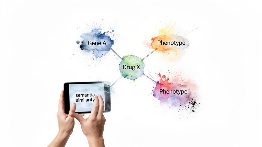
One of the most powerful techniques is calculating semantic similarity. Think of the GO hierarchy as a detailed city map. We can use algorithms to measure the "distance" between the GO terms linked to two different genes. If two genes share very specific, closely related terms—like two addresses on the same block—they are considered functionally similar. This approach often reveals hidden connections that simple sequence comparisons would completely miss, making it a go-to method for predicting protein interactions and flagging new disease-related genes.

Constructing Knowledge Graphs for New Discoveries

The organized, hierarchical structure of Gene Ontology is a perfect backbone for building massive biomedical knowledge graphs. These aren't just static databases; they are dynamic, interconnected webs of information. We can weave together GO data with other critical sources, like drug-target information, protein interaction networks, and clinical phenotype data from OMOP.

Once built, we can unleash graph-based algorithms on these networks to hunt for new patterns. This could mean finding new uses for existing drugs (repositioning) or predicting the real-world impact of a patient's unique genetic mutations. For the complex AI workflows that navigate these graphs, understanding concepts like smart routing AI models is key to making the process both efficient and accurate.

In these knowledge graphs, Gene Ontology provides the crucial "why." It's the functional context that bridges the gap between a gene's role at the molecular level and what we see in the clinic.

The Power of Integrating Ontologies

Looking ahead, the most exciting developments involve weaving Gene Ontology together with other major biomedical ontologies. The partnership between GO and the Human Phenotype Ontology (HPO) is a game-changer. By connecting a gene’s biological process (from GO) to a specific disease symptom or trait (from HPO), we can draw a direct line from molecular glitch to clinical outcome.

This kind of integration is the bedrock of precision medicine. It’s how we’ll move toward therapies designed for an individual's unique genetic profile. Digging into these deep connections involves some advanced methods, which you can read more about in our guide to semantic mapping for healthcare data.

Expert Tips for Advanced GO Applications:

Pick the Right Similarity Score: There isn't a one-size-fits-all metric for semantic similarity. Algorithms like Resnik or Lin work differently, so choose one that best fits the biological question you're asking.
Combine Your Data: Don't rely on GO alone. Its predictive power skyrockets when you layer it with other data types, like gene expression levels, protein structures, or patient records from an OMOP CDM.
Think Programmatically: To build and query knowledge graphs at any real scale, you need to access the data programmatically. SDKs are your best friend here. For instance, the OMOPHub SDKs for Python and R are built to handle exactly these kinds of tasks.

Frequently Asked Questions About Gene Ontology

As we wrap up our deep dive into Gene Ontology, let's tackle some of the most common questions that pop up. Thinking through these points will help solidify how GO works in the real world and how you can apply it effectively.

How Is Gene Ontology Different From a Pathway Database Like KEGG?

This is a great question because it gets to the heart of what makes GO unique.

Think of Gene Ontology as describing the individual 'job titles' and 'skills' of gene products. It tells you their molecular function (what they do), their cellular location (where they work), and the broader biological processes they contribute to. In essence, GO defines what a gene product is capable of.

A pathway database like the Kyoto Encyclopedia of Genes and Genomes (KEGG) is more like an organizational chart or a detailed workflow diagram. It lays out how groups of gene products collaborate in a specific sequence to carry out a complex task, like a metabolic pathway.

So, GO tells you a specific protein is a 'wrench' (its function), while KEGG shows you the entire 'assembly line' where that wrench is used. They are highly complementary, and you'll often use both to get the complete biological story.

Can I Use Gene Ontology for Non-Model Organisms?

Yes, absolutely. One of the most powerful features of the Gene Ontology is that it was designed to be species-neutral. The GO terms themselves—like 'DNA binding' or 'cellular response to heat stress'—are universal biological concepts that apply across the tree of life, from bacteria to humans.

The real difference comes down to the annotations, which are the specific links connecting genes from a particular organism to these universal GO terms. Well-studied model organisms like mice or yeast have a wealth of annotations backed by direct experiments.

For less-studied species, many annotations are generated through computational predictions, often marked with the 'IEA' (Inferred from Electronic Annotation) evidence code. This is perfectly fine, but it's crucial to be aware of the evidence behind the annotation to gauge your confidence in the finding.

What Are Common Mistakes in GO Enrichment Analysis?

GO enrichment analysis is an incredibly powerful technique, but a few common mistakes can easily lead you to the wrong biological conclusions. Steering clear of these pitfalls is essential for getting meaningful results.

Here are the top three to watch out for:

Using the Wrong Background Gene List: This is probably the single most critical error. Your list of interesting genes must be compared against the correct "universe"—that is, all the genes you actually measured in your experiment (e.g., all genes expressed on a microarray), not the entire genome. Get this wrong, and your statistics will be skewed.
Ignoring Redundant Terms: The raw output from an enrichment tool can be a massive list of highly similar GO terms, making it hard to see the forest for the trees. Look for tools that can summarize these results, perhaps by clustering related child terms under a single, more general parent term. This helps reveal the major biological themes without getting lost in the details.
Forgetting to Correct for Multiple Testing: When you test thousands of GO terms at once, you're bound to get some false positives just by random chance. You absolutely must apply a statistical correction for this. Methods like the False Discovery Rate (FDR) are standard practice. Always base your conclusions on the corrected p-value (often called a q-value), not the raw one.

Tip: Programmatically managing GO and other terminologies in your data pipelines can be a real headache. A managed vocabulary service can offload the complexity of versioning, mapping, and updates. To see how this works in practice, you can explore the OMOPHub SDKs for direct programmatic access.

Managing complex terminologies like Gene Ontology is a major infrastructure challenge. OMOPHub eliminates this burden by providing developer-first SDKs and REST APIs for instant, compliant access to standardized vocabularies, letting your team build robust data pipelines and analytics without the overhead of hosting a local database. Learn more at https://omophub.com.

A Developer's Guide to Gene Ontology in Clinical Data